Train Log: s4-dx7-vc-fir-00
Check over here for the code for the release that goes along with this discussion.
The Yamaha DX7 is a classic synth from the 80s, and while it was a masterpiece in its day, it’s starting to show its age, a few of the issues I’m seeing a) You can’t run one in a datacentre - everyone knows cloud is the future c) FM..so last century - the future is DL baby d) MIDI input - sometimes you just wanna break free of those clumsy MIDI controllers
So after back-filling the requirements to the thing I already implemented…what are we doing here today? We’re going to use Deep Learning (DL) to create model to approximate the function of the DX7. Given the beefy requirements needed to train audio models the cloud is a must so tick that box. Finally, transforming the raw MIDI sequence directly to audio would imply quite a bit of extra complexity, since there is no trivial mapping between the MIDI messages index and the real time value in seconds, a simpler solution is to render the MIDI using a sine-wave generator, thus resulting in a simple problem of transforming one soundwave into another.
A sine-wave generator might be possible to implement (probably?) but I am lazy, so instead I constructed a DX7 patch that is as close as possible…So if you want to get really technical were training a DX7 voice conversion (VC) model. I hope you can all follow :|
Dataset
For the dataset we will use 2.5 second audio clips generated by Dexed, a Yamaha DX7 emulator. To drive the synth we will pull 4 beat melodies from the Lakh dataset. I have previously extracted the notes for this dataset and saved them to nintorac/midi_etl on Hugging Face. At time of writing only 2/16 partitions have been generated, however this still gives around 80 million individual note events. we will, however, need to do some processing to get them into a form in which they can be read by Dexed.
The following is a rough overview of the data transformation pipeline.
- aggregate into 4 beat phrases
- gather statistics over those filters
- produce a filter over phrases to remove items that aren’t melodies
- synthesize the phrases using the two voices
1-3 are simple and can be done with a few simple SQL transforms and about 5 minutes of processing, check out the implementation over on Github at Nintorac/s4_dx7/s4_dx7_dbt/models. The files of interest are phrase_stats and the phrase_stats_sub subfolder, melodies and 4_beat_phrases.
Step 4 however is a little more nuanced, a single 2.5 second sample from the dataset takes about 0.5 second to synthesize, and the output is a 44KHz, 16-bit raw audio waveform lasting 2.5s, it consumes 220.5 kilobytes, we could compress to reduce this number but that is another trade-off as the compression process would increase the processing time and either not be super effective or decrease the quality, at this size just 4,535 samples per GB. Not to mention the combinatorial effects of different bit rates, sampling rates.
To work around this we produce the MIDI as a JSON string as an offline preprocessing step, and then online in the training data loader we perform the synthesis. Luckily synthesis is easily parallelised. This gives us the flexibility to choose the synthesis parameters at runtime and reduces storage requirements at the expense of a more complex dataloader.
Model architecture
In this first attempt we want to simplify as much as possible, for that we will model the DX7 as a Finite Impulse Response (FIR) filter. A FIR filter is characterised by the fact that the output of the filter can only depend on its current and previous inputs. This as opposed to an Infinite Impulse Response (IIR) filter where the output of the filter is also used as an input creating a feedback mechanism.

So for the x[n] this represents our input signal, the one we defined to be approximately a sine wave at the given frequency, and y[n] is the target voice signal which is some other voice patch I chose that sounded interesting. (quick note…not totally sure if its valid to describe the network in this way but I think it holds, would be keen for feedback if anyone thinks otherwise, a Github issue would be the best avenue)
How will we implement b? Lets go max-hype and choose a State Space Model (SSM), these have been in the limelight as the potential transformer killer and audio is a killer to a transformers (performance) so lets check it out! Lets also quickly define y_hat as the output of the SSM, i.e \(b_N(x)=\hat{y}≈y\)
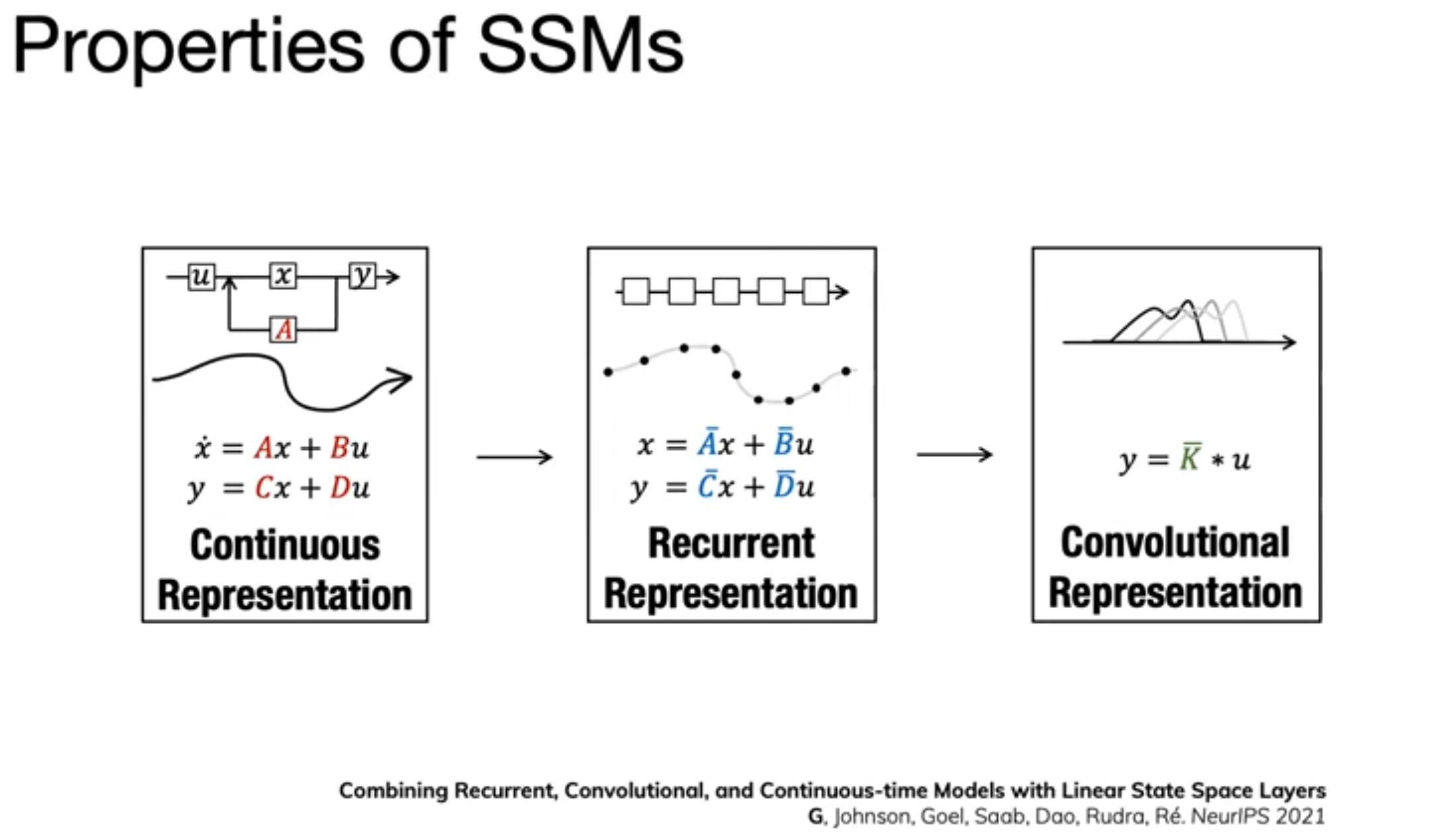
SSMs, which come from the dynamical systems branch of mathematics, are a special kind of function that can be represented in three different ways.
Structured State Space Models for Deep Sequence Modeling (Albert Gu, CMU) - Youtube
The continuous representation while not useful for any applications in my mind right now, does provide a nice theoretical framework to work from since natural audio is a continuous process. Such a prior being built into the network reduces the data requirements.
The recurrent representation would allow for real time application of the filter, again in theory useful, in practice audio implementations in hardware do not work that way and require a bit more work for the network to be hardware-aligned.
Finally the convolution representation, this facilitates efficient training since all steps of the sequence can be calculated in parallel. This is ideal for training since the fewer serial operations we have in the network graph the more data we can throw through it and the faster we’ll have our models. And as a hint to the problem presented in the previous paragraph, it’s also the way real-time software filters are typically implemented.
SSMs by themselves are unstable and difficult or impossible to train, but Structured State Space Sequence (S4) models (see also The Annotated S4) comes along to fix that by defining specific initialisation methods that put the models in a regime where the are much more susceptible to learning. These are the first SSM models to perform well, however they have a property known as linear time-invariance, this is an issue since for example they are incapable of in-context learning (in theory, maybe if it was big enough??). Since the computation from input to output is time-invariant or the same for all time steps it is unable to change its behavior based on prior inputs.
Mamba solves this problem by including some input conditional computation step to each time step, usually this would blow up memory requirements but they implement some neat hardware aware tricks to make it possible.
I ended up choosing the S4 model since I wanted to test some intuitions on how the linear in variance would make the model respond when it has only only a linear response to the past, specifically I am wondering if the model will generalize to polyphony>1 when it has only been trained on melodies. Also it is conceptually and computationally simpler.
This video is extremely good at providing a lot of the foundations needed to understand these models, I highly recommend it!! Mamba and S4 Explained: Architecture, Parallel Scan, Kernel Fusion, Recurrent, Convolution, Math - Umar Jamil
Training Regimen
For the most part (all of it) the S4 code was stolen from the official implementation , to this I hacked in the previously described dataset and used the +experiment=audio/sashimi-sc09 preset. All the default training options were used.
The dataset was limited to the first 20k samples (since the dataset contained 18100 samples this has no effect). The synthesis parameters consisted of the sample rate at 8000 and the bit rate at 8. The batch size was configured at 14 as this was the largest that could fit on the GPU. Gradient accumulation was set to 2, resulting in an effective batch size of 28 (more or less?).
The model was trained for >100k steps and manually stopped since gains were plateauing and results were good enough™
Training took ~4 days with an approximate time per batch of 1.3 seconds.
Training details
Training was performed using a Lambda Labs A10 instance, the final cost of the training session came in at $65AUD($42USD).
I was unable to find any carbon usage information from Lambda Labs, so can’t comment on that.
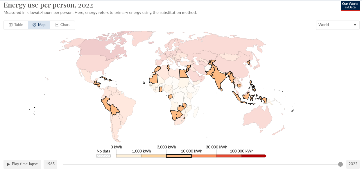
The best I can get at the point is to observe the GPU power usage, as reported by Weights and Biases, and on rough estimation of 90 hours of training @ 140W mean consumption results in 12.6kWh, which is about dead on the energy density of 1L of petrol. Since we don’t know the consumption of the machine itself lets assume ~560W which conveniently puts us at 5L petrol consumed to train.
Here is a list of countries where the per capita energy consumption matches the energy consumption needed to train this model. It’s not totally clear and I had a bit of a hunt for the answer…but I hope this is daily usage not yearly.
Through another lens though which to view this usage is via that of CEO-Jet-Hours (CJ/h) in which case were clocking in at between 1/730 and 1/820 CJ/h (cruisng fuel usage at energy density of petrol) at cruise.
According to the drivingtests.nz, 1kg of petrol would release 2.3Kg carbon, next carbon offsets on the European Carbon Credit Market are going for €60/tonne. So we need around 5*2.3*60/1000=0.69 so 0.69c (lol) to offset the train. I’ve tried to make this all worst-case scenario here and hope the energy sources are a little cleaner than that. I’ve purchased some native seeds and spread them around to relieve the impact my conscience.
Anyway, guilty sidetrack over, lets move on.
Results
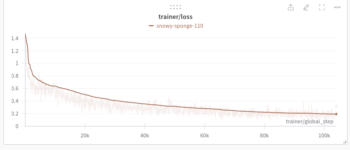
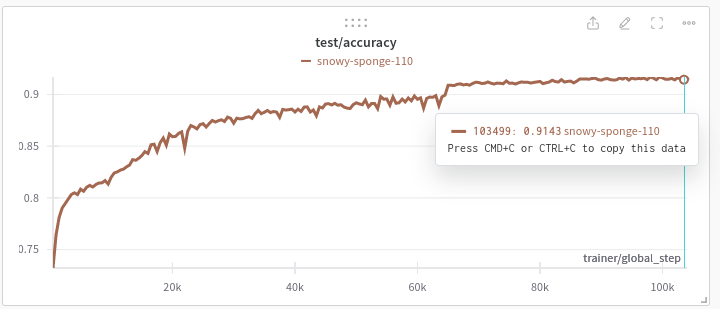
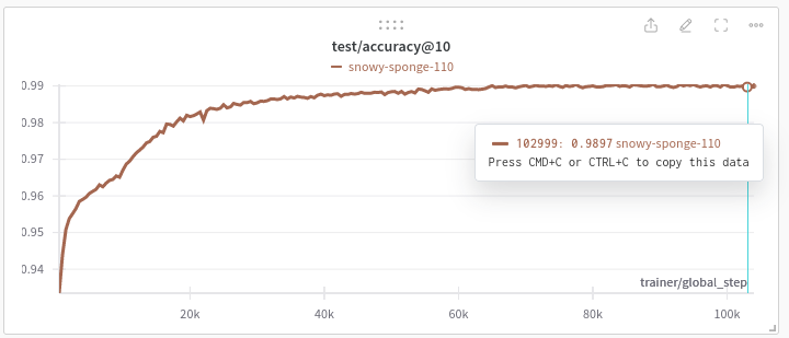
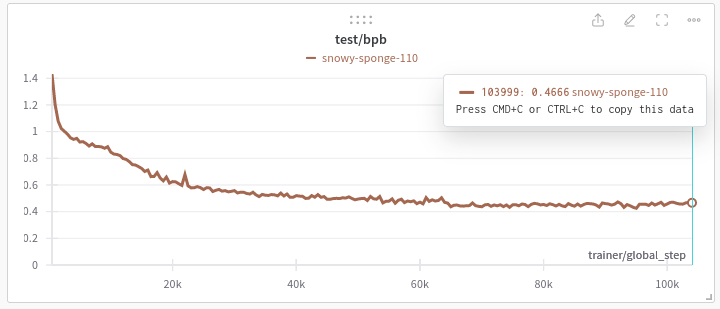
Here are the loss curves for the model, the trainer loss is nice and smooth. The test/accuracy you would expect to be a bit choppy as it’s very sensitive to minor perturbations in model output. The step observed at ~70k steps was a result of the learning rate dropping.
Evaluation
Work to be done here, there are large range of visualizations I would like to see here and producing them all will take time and effort, which feels wasted on a broken model (details on that in the Bugs section), instead here are some ad-hoc visuals and some explanations.
Below is a graph of the transformations for this model/dataset. Each of the nodes is a type of data, each of the edges is a function. You can hover over the edges to see a representation of that nodes data, these are images, audio streams or in the case of the MIDI node a file download.
If you find it difficult to see a plot for a node pan the graph scene so the node is in the top right of the page. Best viewed on a PC but kind of works on mobile too. Clicking through the to the link will make it much bigger.
Click here to see the full screen application
Node descriptions
- MIDI - the MIDI file that defines the sequence of notes
- Source Signal - the MIDI rendered in the source voice
- Target Signal - the MIDI rendered in the target voice
- Corrupt Source Signal - the source signal, corrupted to match the implementation used to train this model
- Corrupt Target Signal - the target signal, corrupted to match the implementation used to train this model
- Clean Source Generated Signal - the generated signal when using the real source signal, the source signal is out of distribution (OOD) and the output does not show any structure. Interesting that it chooses silence in this situation over noise
- Corrupted Source Generated Signal - the generated signal when using corrupted data as the input, this is what is was trained on, it matches quite closely with the Corrupt Target Signal
I was pretty happy with the way the above turned out though it was an extremely manual process so given some automation these types of visuals could make a great debugging tool. See the code to produce it here
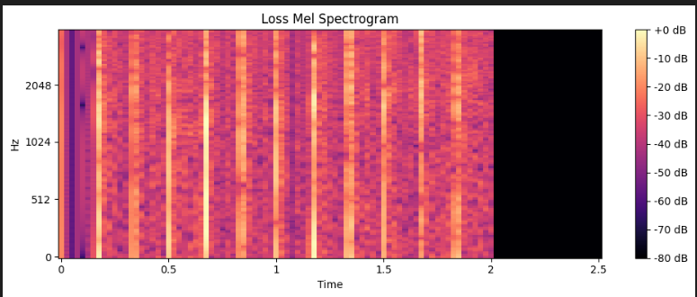
Finally, here is a mel-spectrogram depicting signal found by subtracting the models target signal from the models outputs (y-y_hat), as you can see there are noise peaks across the full spectrum at regular intervals. This example is the same as the one used in the prior visual. These noise peaks coincide with note changes, these would hopefully be fully alleviated by removing the auto regressive offset (described in the bugs section), and at the least will be reduced.
Bugs
Here are a list of issues that I noticed after training, note these issues have been left in place for posterity in the source release associated with this post.
- The polyphony calculation has an off by 1 error
The polyphony is being calculated as the maximum number of notes occurring at the same time as a given note. This comes out at 1 for each of the notes if they occur simultaneously. As such the model was trained on all midi tracks with exactly polyphony of 2 instead of melodies.
This would likely have a large impact and make the problem much harder to solve, since it now needs to learn what all combination of notes sound like, we limit the note range from A0 to C8, this gives 87 uniques notes and therefore the space we need to learn, ignoring temporal dependencies, is now
87 Choose 2 = 3741rather than 87 which it would have been otherwise. - Both the source and target signals were rendered three times per dataset iteration The GPU was maxed out for most of the training run, so it did not result in too much of an issue. However this likely would have resulted in larger warmup times between epochs. The upside of this though is it goes to show how much headroom the dataset has over the model, which is to say the dataset should be able to scale to much larger models smoothly.
- The source and target signals are auto-regressively shifted
- This probably doesn’t harm anything, but it will mean that the model will take at minimum one sample to react to changes in the source signal (eg. a new note is start), in practice there is likely little perceptual difference between these two. On the plus side there is likely free gains to be had removing this offset.
- The dataset was limited to only source MIDI files who’s ID (i.e file hash) began with a ‘f’ At time of training only e and f are available anyway, so we basically halved the dataset size. There was some level of overfitting observed which a larger dataset may help to mitigate.
- The dataset was incorrectly calculating the bit crushing, this also resulted in the waveform offsetting and truncating at 1 This essentially results in a bit-rate reduction of 2x for the bit-crush off by 1, and another 2x since half the waveform is removed. Although for the second point I’m not so sure since the DX7 is so regular in the waveform its generating (at least for the patches from this experiment)
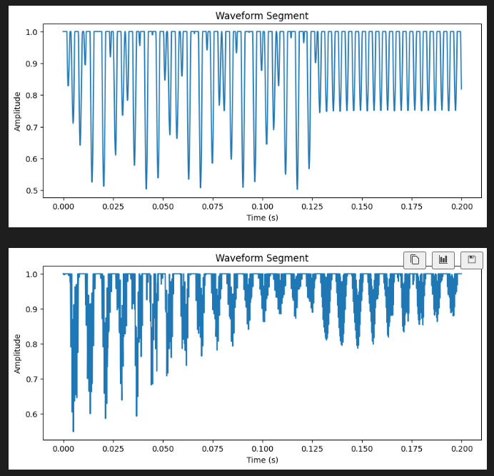
Waveform visualizations of the corrupted target signal used during training.
Some other scattered notes
Improvements
Apart from fixing the bugs, here are a few things to fix for the next round
- Smaller network
- Both in time and size
- time to the maximum note duration + the release duration
- release duration is how long the note lasts after release
- the chosen target patch was chosen to have short release
- Will start small and work my way up
- time to the maximum note duration + the release duration
- Both in time and size
- Define the train test split in the data pipeline
- Implement some kind of double buffering around the dataloader
- Lots of utilisation drops between epochs as dataloaders spool up.
- Would be cool if there was a setting to warmup the concurrency here,
- early concurrency creates too many jobs which fight for resources, later stage pipelines jobs get starved out and it takes some time to clear the early stages resulting in a fast spool up
- we could alleviate if there was a way to prioritise jobs a the partition level
- if we let the initial partition complete before launching further jobs that would likely be enough as well, at least for my use cases
- Some refactoring to ensure all transform paths are using the same core logic
- At the same time, swap out self implemented transforms for library alternates. i.e how I could have avoided training on the wrong data
Future Directions
These are ideas for improvements and experiments that I don’t plan for yet but think would be interesting, likely to be geared towards more beautiful solutions rather than practical ones ;)
- Continuous inputs
- Using something like Fourier Features should do the trick here
- Simplifies the data pipeline
- Supports arbitrary bit rates without architectural changes
- Continuous outputs
- Simplifies the data pipeline
- A better prior than the current categorical targets since we are targeting a continuous variable
- Arbitrary bit rates
Closing thoughts
I’m a bit sad about the data corruption, I had visualized the spectrograms and listened to the samples prior to training, I suspected something was amiss but didn’t dig enough and hadn’t added the waveform plots as a visualisation method.
Other than that I am feeling quietly confident, this model has very little issues learning this transform and I’m feeling good about it’s ability to generalise to multiple voices.
I can produce 2.5 seconds of audio in ~1 second and increasing the batch size doesn’t have much effect so we have a real time factor (RTF) < 1 when using the convolutional form, is pretty fast. However, since we produce 2.5s@8000hz this is an effective buffer window of 20,000 samples, resulting in very high latency. If we scale this down to a more normal processing buffer window size of 256/512 its not clear that we would be so lucky..and that’s assuming that you can chain sub-kernels of the full SSM filter which is not totally clear!
Finally, in terms of affordability things have come a long way, when I wrote my DX7 patch generator V100s were at $2.55/hr (Salt Lake City in October 2000 [1]/ [2]/). With more limited capability and memory compared to the A10 the training would have taken longer, and I would have needed to train on one of the big cloud providers who dig you with all kinds of other associated costs, eg the machine needed to run the GPU. I would roughly estimate ~10x at reduction in cost over that time.
Also, shoutout to Lambda Labs the real MVP here, transparent pricing and no issues in my experience! Though I will say it is a bit difficult to work without a persistent machine image and availability can be a bit hit or miss though. Maybe that’s a good thing, the temptation to deploy an 8xA100 is high! (not sponsored content)
Anyway keen to explore more! There’s a lot to get into!