The RADDD Stack: Implementation
Today I will describe how to produce an all local data platform using the RADDD data stack (everyone’s talking about it, promise), the stack consists of 4 layers that work together to provide a fast, tunable platform that can scale to production seamlessly.
For a more detailed description of the stack see the accompanying article found here
If you just want to see what we actually produce from this pipeline go checkout this site where I render the melspectrogram and a player for the audio sample. Beware! This is running in a Google Cloud Run and can be slow on the first load!
For a random sample refresh on this page dx7.nintoracaudio.dev/phrases/0, or you can choose a specific sample by setting a number greater than 0 in the above URL. eg dx7.nintoracaudio.dev/phrases/99
Stack
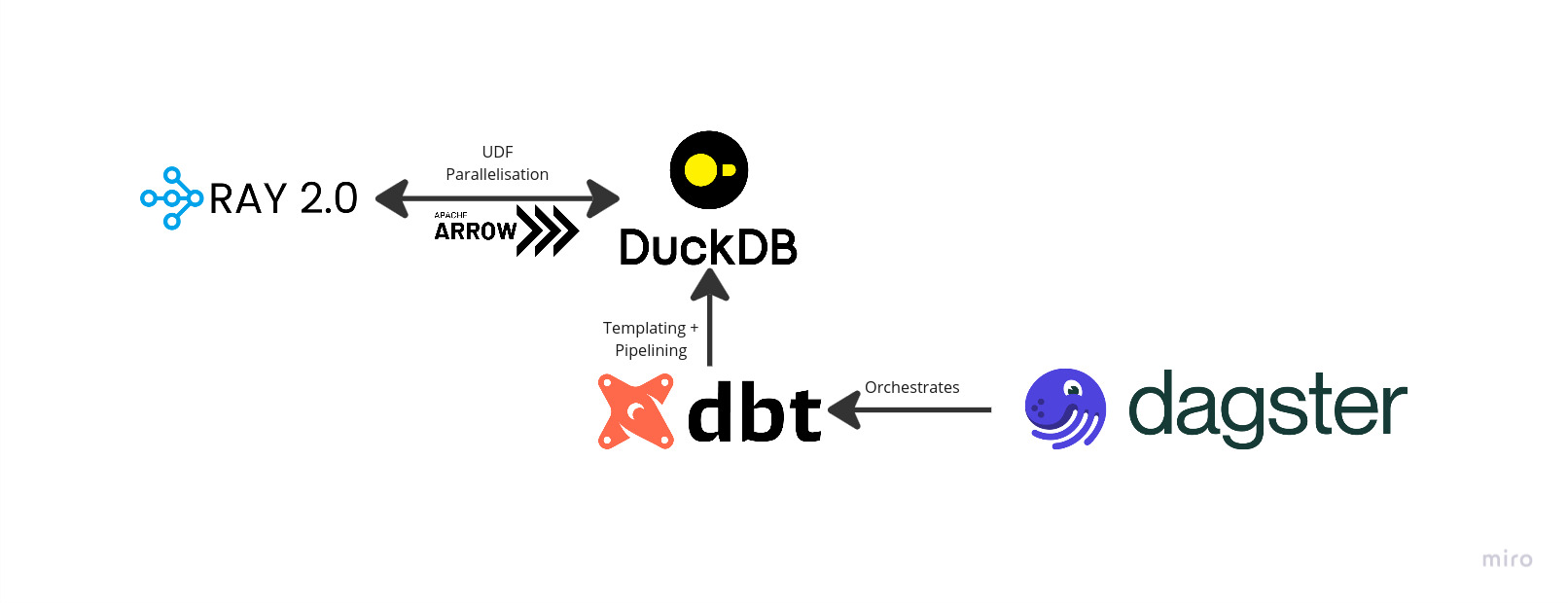
Here’s a quick diagram to show how everything ties together
Problem Space
For this example we are going to explore the Lakh Dataset and work on building an application that can reliably reproduce a synthesized audio dataset. I am going to break out an old favorite of mine Dexed to use as the synthesizer and Spotify’s Pedalboard as the VST host.
As source data I have pulled a table detailed_notes, that is derived from the Lakh dataset, you’ll have to trust me on its origin, maybe I’ll write about it sometime.
CREATE TABLE lakh_dataset.midi_music.detailed_notes (
	midi_id VARCHAR, -- hexidecimal uuid of the MIDI song
	track_id VARCHAR, -- hexidecimal uuid of the MIDI track
	message_id VARCHAR, -- hexidecimal uuid the MIDI message
	start_time DOUBLE, -- start time in beats of the note
	duration DOUBLE, -- duration in beats of the note
	velocity BIGINT, -- the MIDI velocity of the note
	note BIGINT, -- the MIDI pitch of the note
	set_type VARCHAR, -- train, test or validate
	p VARCHAR -- first hex char of the midi_id
);
The code to create them for this is available here but is in somewhat of a state and not documented.
Plan
- Acquire source data
- Initial DBT configuration
- Configure profile to load dataset Parquet files as tables
- Configure project to register source tables
- Write SQL DBT models to extract 4 beat samples
- Build note objects to group midi message information
- Aggregate notes into 4 beat groupings
- Write a Python UDF for DuckDB
- Accept an Arrow array of 4 beat MIDI samples
- Use Ray to batch the array and perform the work function
- Consume each 4 beat sample of MIDI messages
- Use Dexed and Pedalboard to render the beats
- Transcode to lossless compressed FLAC format
- Returns sample
- Collated results back into an Arrow
- Return arrow array
- Write a Python DBT model
- Subquery the DuckDB relation to only process a partition of the 4 beat samples
- Register the UDF
- Execute the function over the notes list
- Save the results into the renders catalog
- Configure Dagster
- Load the SQL models as regular Assets
- Load the Python model as a partitioned asset
- Define the Partitions
- Configure the Python model to be incremental
Implementation
NOTE: Before we go too deep don’t take these code snippets as total gospel, the narratives match but the final code may be slightly different, see the repo here for the fully functioning version.
To begin you will need to create your an environment in which you can work in. For me, my go-to is to use conda. Assuming you’ve already got it installed you should then run the following commands
conda create -n raddd python=3.11.2
conda activate raddd
Note: we specifically need 3.11.2 for this, any higher and the VST fails to load, and <3.11 gives an error because of the input type definition when registering the UDF.
Initial DBT configuration
To configure DBT first we will need to install some packages, for this we will need dbt-core and dbt-duckdb which will install the core DBT libraries as well as the DuckDB adapter.
pip install dbt-core dbt-duckdb
With that done, we initiate a new project named raddd_dbt with the following command, when asked to select which database you would like to use choose DuckDB
dbt init raddd_dbt
At this point you should see a new folder created with the raddd_dbt name and it should look like this.
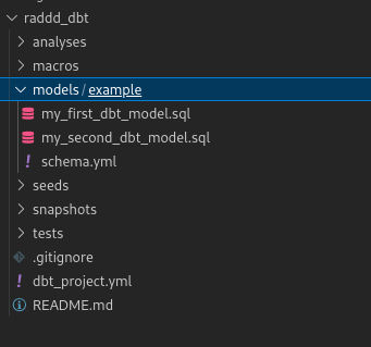
Next we will delete the raddd_dbt/models/example folder and create a sources.yml under raddd_dbt/models, the contents of that file are as follows;
sources:
  - name: midi
    meta:
      external_location: "../data/{name}.parquet"
    tables:
      - name: detailed_notes
And one final piece of setup, we will modify the raddd_dbt profile to save the DuckDB database in a location of our choosing, in this case we want to keep all our outputs in the data folder. First create the file raddd_dbt/profiles.yml and then set it’s contents to the following. Note: the path in the profile is relative to where you are running DBT from so we modify it to look like this.
raddd_dbt:
  outputs:
    dev:
      type: duckdb
      path: ../data/dev.duckdb
      threads: 1
  target: dev
The external location tells the dbt-duckdb adapter to look in a specific location for the sources and the {name} in the path will get substituted with the table name at runtime, see the dbt-duckdb documentation for more information
To make sure everything is working we will cd into the raddd_dbt folder and use the following command dbt run --profiles-dir .. You should see some output that mentions there are 4 sources in the project. eg
02:51:24 Found 4 sources, 0 exposures, 0 metrics, 391 macros, 0 groups, 0 semantic models
Acquire source data
Now before going any further we need some data, we could write a data pipeline that would download the Lakh dataset directly from the source and calculate all the notes but that’s not the point of this so instead lets use some I prepared earlier, they can be found at nintorac/midi_etl . The table there contains all notes from a subset of Lakh, each row contains the pitch, velocity, start time and duration which define the note as well as the track_id which allows us to pull out full tracks with a simple grouping.
To source the data we’re going to use a neat trick afforded by dbt-duckdb and DuckDB, first dbt-duckdb allows us to use DBT source configurations to configure source tables to useDuckDB’s capability to query parquets directly from any https endpoint.
To configure that simply edit raddd_dbt/models/sources.yml to be the following;
sources:
  - name: midi
    tables:
      - name: detailed_notes
        meta:
          external_location: |
            read_parquet(
              [
                'https://huggingface.co/datasets/nintorac/midi_etl/resolve/main/lakh/detailed_notes/p=f/data_0.parquet',
                'https://huggingface.co/datasets/nintorac/midi_etl/resolve/main/lakh/detailed_notes/p=e/data_0.parquet'
              ]
            )
The external_location is simply a query that will be rendered into place. It will be processed by DBT so you can include any jinja or macros in here if you have more complex needs!
Note: if you want to do some analysis on the detailed_notes table yourself, you may want to clone it locally first eg make a model with select * from {{ source('midi', 'detailed_notes') }} and configure it to materialise as a table.
Write SQL DBT models to extract 4 beat samples
Now we are ready to define our query, the table we have to work with gives us detailed_notes which provides the start_time and duration (measured in beats) as well as the track_id. First we create a struct that maps all the necessary information to construct a MIDI note into a single struct, as well as calculating the bucket (which 4 beat section of the track) that note falls into. Finally we do a simple group by over the bucket and perform a list aggregation over the note struct.
We should convert the beat basis notes onto a real time basis, to do this we calculate the real time value as time*(60/bpm), so if we want 60BPM, then we must multiply all time values by time * 60/60 = time * 1. Hmm, guess it’s on a real time basis already, nothing to do here.
Here is the query, which should be written to raddd_dbt/models/4_beat_phrases.sql.
with note_dicts as (
	SELECT
		floor(e.start_time/4) bucket
		, e.track_id
		, {
			'start_time': round(e.start_time-bucket, 2)
			, 'duration': round(e.duration, 2)
			, 'velocity': e.velocity
			, 'note': e.note
		} note
	FROM {{ source('midi', 'detailed_notes') }} e
	order by e.track_id, e.start_time, e.note, e.duration, e.velocity asc
)
select bucket, track_id, list(note) notes from note_dicts
group by bucket, track_id
One important thing to note in this file is {{ source('midi', 'detailed_notes') }} which doesn’t look much like the SQL you know and love. Here we are providing a template string that DBT will detect and replace with the appropriate information, specifically we are referncing the detailed_notes table from the source database midi we declared earlier in sources.yml.
At this stage you should be able to deploy this table to the DuckDB database with dbt run --profiles-dir . but we’ll skip that for now and do it in a later stage.
Write a Python UDF for DuckDB
This section has a few moving parts, but lets start with a definition for a user-defined functions (UDF), that is a function that will be executed by your database process that is written in the language of your choice, in this case we’re using DuckDB to call Python code.
So, onto the business logic, that is turning the notes list into a FLAC file. For that we are going to need two extra libraries, namely pedalboard which hosts the synthesizer plugin (VST), mido which is a low level library to play to create MIDI and pydub which handles transcoding the raw waveform down to FLAC. Let’s install them;
pip install pydub pedalboard mido
We’re also going to need to download the VST, you can find it on the Dexed release page and on that page you should download and unzip the dexed-0.9.6-lnx.zip archive. Once extracted create a new folder at the root of the directory named instruments and copy the Dexed.vst3 sub-folder into it.
Next we need to do the following steps; 1. Turn the notes list into a set of MIDI events 2. Load the Dexed VST into a pedalboard instrument 3. Render the midi notes with the instrument 4. Transcode the raw waveform into FLAC
Here’s the code
def to_midi(notes: List[dict], transpose:int=0)->List[mido.Message]:
	# the note's are represented as start_time, duration. But MIDI needs note_on, note_off tuples, so each note event will produce two MIDI messages
    return list(chain(*[
            (Message('note_on', time=note['start_time'], note=note['note']+transpose, velocity=note['velocity']),
             Message('note_off', time=note['start_time']+note['duration'], note=note['note']+transpose, velocity=0)
             ) for note in notes]))

def render_notes_list(notes: List[dict])->bytes:
    instrument = load_plugin("../instruments/dexed-0.9.6-lnx/Dexed.vst3")

	notes = to_midi(notes)
	x = instrument(
        notes,
        duration=5, # render 5 seconds of audio
        sample_rate=sample_rate, and included some tracing information,
	)

	x = pydub.AudioSegment(
		x.tobytes(),
		frame_rate=sample_rate,
		sample_width=x.dtype.itemsize,
		channels=2
	)
	with NamedTemporaryFile('rb+') as f:
		x = x.export(f.name, format='flac')
		x = f.read()

	return x
Great, we can render a single list of notes into a FLAC, but there are a few issues. For one we have to reinitialise the VST instrument for every notes list, this introduces needless overheads. Secondly, we plan to use type='arrow' based UDF for DuckDB, this means that the input to our function will take a vector of notes lists (a list of list of notes, where the inner list defines the 4 beats of the track and the outer list is a batch of such sections), For the moment DuckDB will only process one such vector at a time, this leaves only one core on our machines sated for work and the others going hungry. So we must implement the parallelisation ourselves and to do this we utilise Ray.
So first install Ray, we will also need pyarrow and pandas for this step so install those too;
pip install ray pyarrow pandas
Then without further ado, here’s the modified code.
from itertools import chain
from tempfile import NamedTemporaryFile
from typing import List

from mido import Message
from pedalboard import load_plugin
from tqdm import tqdm
import pydub
import ray
import pyarrow as pa
import duckdb


SAMPLE_RATE = 22050

def to_midi(notes: List[dict], transpose:int=0)->List[Message]:
	# the note's are represented as start_time, duration.
    # But MIDI needs note_on, note_off tuples,
    # so each note event will produce two MIDI messages
    return list(chain(*[
            (Message('note_on', time=note['start_time'], note=note['note']+transpose, velocity=note['velocity']),
             Message('note_off', time=note['start_time']+note['duration'], note=note['note']+transpose, velocity=0)
             ) for note in notes]))


@ray.remote
def process_chunk(notes: List[List[dict]])->pa.array[bytes]:

	chunk = notes.to_pandas()
    # Load a VST3 or Audio Unit plugin from a known path on disk:
    instrument = load_plugin("../instruments/dexed-0.9.6-lnx/Dexed.vst3")
    samples = []
    t = tqdm()
    for notes in map(to_midi, chunk):

        x = instrument(
        notes,
        duration=2.5, # seconds
        sample_rate=SAMPLE_RATE,
        )

        x = pydub.AudioSegment(
            x.tobytes(),
            frame_rate=SAMPLE_RATE,
            sample_width=x.dtype.itemsize,
            channels=2
        )
        with NamedTemporaryFile('rb+') as f:
            x = x.export(f.name, format='flac')
            x = f.read()
        samples.append(x)
        t.update(1)

    return pa.array(samples)

def process_batch(batch: pa.array[List[dict]])->pa.array[bytes]:

    rows_per_batch=max(10, batch.length()//32) # max of size 64 batches @ 2048 sized vectors
    chunks = []

    for chunk_start in range(0, batch.length(), rows_per_batch):

        chunk = process_chunk.remote(batch.slice(chunk_start, rows_per_batch))
        chunks.append(chunk)

    return pa.concat_arrays(ray.get(chunks))
The function render_notes_list has been modified into process_chunk which is a ray.remote function, that takes a batch of 4 beat sections, initialises a single instrument and processes them each into FLAC bytes sequentially. And we’ve added a procces_batch function, this takes a pyarrow array that is the vector supplied by DuckDB and breaks it into discrete jobs that can be processed in parallel.
Ideally we pull this bit of logic into a module by itself and reference that within the Python DBT model, however this causes some weird issues with DBT so for now we will just include this code in the DBT model directly. So create a the file raddd_dbt/models/render_midis.py and add the functions in there.
Write a Python DBT model
To write a Python DBT model is very simple, you just create a function named model which takes two arguments that we will call dbt and session. The dbt argument allows us to configure or fetch various things with DBT itself and the session argument which is a DuckDB connection. The dbt object can also configure the DAG itself by way of the dbt.ref function which returns a duckdb.DuckDBPyRelation object.
The first thing to do is pull a reference to the 4_beat_sections model created earlier that will serve as input to the UDF, we use the dbt.ref function to do this.
Next we have to register the UDF into the DuckDB session, the session.create_function facilitates this, you supply a name for the function, a pointer to the function, the input types and the output types, additionally we set the type to arrow so that DuckDB will give us a batch of 4 beat sections rather than just one.
All that’s left now is to run the query that will render the MIDI to FLAC, for that we use session.query which will produce a new DuckDB relation object, inside the query we run the process_chunk function that was created over the notes column and (with the magic of DuckDB) reference the midi object we pulled using dbt.ref.
With that done, we need to convert the flacs relation to an arrow table that will be the output of the table, ideally this wouldn’t have to happen but without it the midi variable goes out of scope and the DuckDB magic breaks.
Here’s the code so far, append it to raddd_dbt/models/render_midis.py;
def model(dbt, session):

    midi: duckdb.DuckDBPyRelation = dbt.ref("4_beat_sections")

    session.create_function(
        'process_chunk',
        process_batch,
        [duckdb.typing.DuckDBPyType(
            list[{
                'start_time': float,
                'duration': float,
                'velocity': int,
                'note': int,
            }
            ]    )],
        duckdb.typing.DuckDBPyType(bytes),
        type='arrow')

    flacs = session.query("""
    select track_id, bucket, process_chunk(notes) from
		    (select * from midi limit 10)
    """)

    return flacs.to_arrow_table()
Note 1: we limit the number of midis to render for now as it’s unlikely your poor little computer could render them all without running out of memory, we’ll come back in the next section to optimise that to allow us to produce the full results.
Note 2: Pylance complains about the input type with the error Dictionary expression not allowed in type annotation which results in some ugly red squiggles in my editor, but the code runs soo…ship it?
Configure Dagster
In order to break the task up into multiple jobs, we must partition our source data and then run the DBT model over each partition. We could manage this manually however it is cumbersome and if a particular partition fails it may not be simple to know that if we just had a script to loop over all partitions. In comes Dagster that can help us orchestrate that. We will need to add the dagster library to facilitate that, as well as the dagster-dbt lib to allow it to talk to the DBT project, let’s install them.
pip install dagster dagster-dbt
Now we need to create the Dagster portion of the project, to do so we will create a module to contain the dagster code, in this example we’ll call it raddd. So cd to the root of the project and create the module like so;
mkdir raddd
touch raddd/__init__.py
To get things going we will first just import the entire DBT DAG of assets all together, to do this we use the dagster_dbt.load_assets_from_dbt_project method, we need to give it the location of the DBT project as well as the profiles directory. To locate those dirs we’ll use pathlib and since there isn’t much code here we’ll just shove it all in the __init__.py and call it a day, here’s the code;
from pathlib import Path
from dagster_dbt import load_assets_from_dbt_project

project_root = Path(__file__).parent / '..'
dbt_project = project_root / 'raddd_dbt'
assets = load_assets_from_dbt_project(
    dbt_project.as_posix(),
    profiles_dir=dbt_project.as_posix(),
)
Simple, with this all in place we should be able to finally run the project! To do that we’re going to need to launch the dagster-webserver (we will also need to install it), and we will use the -m flag to point it at the module we defined. So cd into the project root again and run the following command;
pip install dagster-webserver
dagster-webserver -m raddd
Then open up the Dagster frontend, usually found at localhost:3000 and you should see the DAG you defined in DBT and that should look a little something like this;
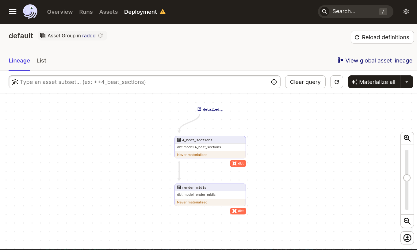
Note 1: Sorry, Dagit has no no dark mode :( (or me :|)
Note 2: You can ignore the yellow triangle on Deployment, until you try to launch a backfill
Great click Materialize all in the top right corner and it will kick of a run of the graph, first extracting all 4 bar sections of the source table and then rendering the first 10 sections from that table. OK but we could have done that with DBT directly*, so lets integrate a bit deeper with Dagster now so that we can render the whole dataset without running out of memory.
First we’re going to need to define a partition, in this case we will add a column to the 4_beat_sections, we want the partitioning to match the in memory layout of the dataset, this will help increase the efficiency of the vectors in DuckDB (filters can occur per vector, if this happens you can have sparsely filled vectors which incurs extra memory access overheads). To do this we can use the ntile function of DuckDB, it takes an integer as input and then evenly distributes a value between 1 and that integer among the rows, finally order by that value and the requirements are met. We should materialise this table to take advantage of the memory savings, too. More on that later.
with note_dicts as (
	SELECT
		floor(e.start_time/4) bucket
		, e.track_id
		, {
			'start_time': round(e.start_time-bucket, 2)*0.5
			, 'duration': round(e.duration, 2)*0.5
			, 'velocity': e.velocity
			, 'note': e.note
		} note
	FROM {{ source('midi', 'detailed_notes') }} e
	order by e.track_id, e.start_time, e.note, e.duration, e.velocity asc
)
select
	bucket
	, track_id
	, list(note) notes
	, ntile({{ var('n_partitions', 100) }}) over () as p
from note_dicts
group by bucket, track_id
order by p
Here we have created a DBT variable using env_var and given it a default value of 100, this will be the number of partitions, later we will use Dagster to set this variable.
Next is to update the render_midis model to only select the phrases in a particular partition, we use the same technique by referencing a var in DBT. Here’s the code;
def model(dbt, session):

    midi: duckdb.DuckDBPyRelation = dbt.ref("4_beat_sections")
    partition_n = dbt.config.get('partition_n', 0)

    if partition_n is None:
        raise ValueError("Must configure 'partition_n' var")

    session.create_function(
        'process_chunk',
        process_batch,
        [duckdb.typing.DuckDBPyType(
            list[{
                'start_time': float,
                'duration': float,
                'velocity': int,
                'note': int,
            }
            ]    )],
        duckdb.typing.DuckDBPyType(bytes),
        type='arrow')

    flacs = session.query(f"""
    select track_id, bucket, process_chunk(notes) flac_bytes from
		    (select * from midi where p={partition_n})
    """)

    return flacs.to_arrow_table()
Note: the sub-select must be in brackets otherwise process_chunk is run over everything and only then filtered.
We now consume a variable named partition_n and use this to filter the MIDI phrases, if you materialize the the Dagster assets now you will get a very fast run, since we default to 0 for the partition_n and the ntile function from before starts at 1. At least we can make sure the code still runs!
Next we must modify Dagster to supply the correct variables for the correct partition. In order to achieve this we’re going to have to break the asset loading step into two stages, one for the partitioned asset, the other for the non-partitioned asset. Then we define a StaticPartitionsDefinition, to this we supply a list of all the possible partition values, somehow we must also make this line up with the n_paritions variable in the 4_bar_phrases query. For this we will use an environment variable for lack of a better idea, it’s possible we could use the DynamicPartitionsDefinition but that’s left as an exercise to the reader.
Here’s the new code for raddd/__init__.py;
from itertools import chain
import os
from pathlib import Path
from dagster import Definitions, StaticPartitionsDefinition, with_resources, configured, AssetsDefinition
from dagster_dbt import load_assets_from_dbt_project
from dagster_dbt import dbt_cli_resource as dbt

project_root = Path(__file__).parent / '..'
dbt_project = (project_root / 'raddd_dbt').as_posix()
N_PARTITIONS = os.environ.get('N_PARTITIONS', 800)

# Load static assets
assets = load_assets_from_dbt_project(
    dbt_project,
    profiles_dir=dbt_project,
    select='4_beat_phrases',
)


# Load partitioned assets
def partition_f(partition):
    return {'partition_n': int(partition)}

def metadata_fn(x):
    return {"partition_expr": "p"}

# list of strings for each partition
partitions_def = StaticPartitionsDefinition(list(map(str, range(1, 1+int(N_PARTITIONS)))))

partitioned_assets = load_assets_from_dbt_project(
    dbt_project,
    profiles_dir=dbt_project,
    select='render_midis',
    partitions_def=partitions_def,
    partition_key_to_vars_fn=partition_f,
    node_info_to_definition_metadata_fn=metadata_fn
)


assets = with_resources(
    chain(assets, partitioned_assets),
    resource_defs={
        'dbt': dbt.configured({
            'profiles_dir': dbt_project,
            'project_dir': dbt_project,
            'vars': {'n_partitions': N_PARTITIONS}
        }),
    }
)

defs = Definitions(
    assets=assets,
)
In the partitioned section we define two extra functions, partition_f which figures out how to translate the Dagster partition element to config that will be supplied to DBT and the metadata_fn that tells Dagster which column to look at when loading the partitioned asset in downstream steps (not that we have any in this case).
The final thing to do is let DBT know not to delete the table on a rerun, to do this we must set the materialization strategy to incremental. While we are there we should also configure the 4_beat_phrases model to build a table as by default it deploys as a view which would potentially interfere with the partitioning optimizations. You can also delete the example configuration created by the DBT templater. To do this we edit the dbt_project.yml file and modify the models key. It should look like this after the change;
models:
  raddd_dbt:
    +materialized: table
    render_midis:
      +materialized: incremental
And there we have it, partitioning fully implemented and if you wanted you could now materialise the full table using the Dagster UI, that is not reccomended without first configuring the dagster-daemon and limiting it to 1 concurrent run. For now though you can try to materialise a single partition to verify it’s working. Click the materialise button again and select a single partition in the popup that appears.
Improvements
- Deduplicate the sequences
- Filter out drum sequences
- Allow passing in a sysex defining the DX7 patch settings
- At this RTF it’s probably viable to generate on the fly for ML pipelines
- Scale out with a Ray Cluster and run faster